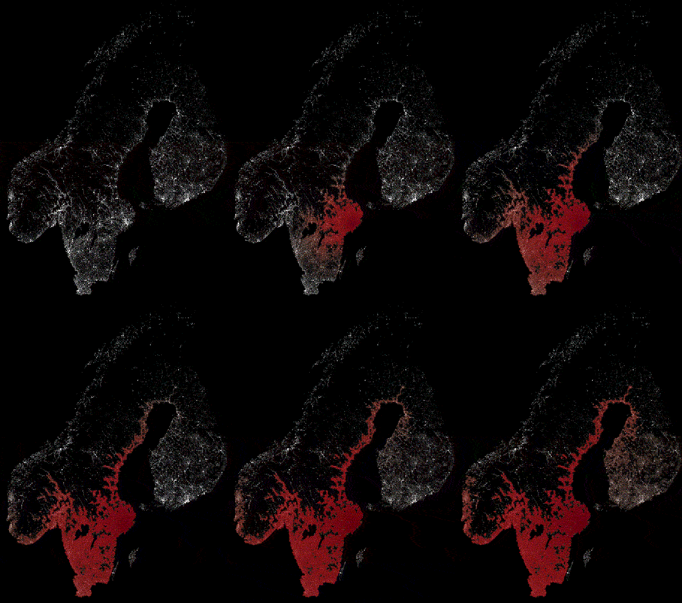
Model of a zombie outbreak in Sweden, Norway and Finland (Denmark is fine)

alt text

The spread of infection as a gif. Even the Finns will succumb.

Inspired by Jason at Almost Looks Like Work I wanted to take on some modeling of disease spread. Note that this model has no claim what so ever on reflecting reality and is not to be mistaken for the horrible epidemic in West Africa. On the contrary, it’s more to be viewed as some sort of fictional zombie outbreak. That said, let’s get down to it!

$\begin{align} u(t) & = \begin{pmatrix} S \\ I \\ R \end{pmatrix} & f(u) = u'(t) = \begin{pmatrix} S' \\ I' \\ R' \end{pmatrix} = \begin{pmatrix} -\beta I S \\ \beta I S - \gamma I \\ \gamma I \end{pmatrix} \end{align}$

This is what’s called a SIR model where the letters S, I and R reflects different states an individual can have in a zombie outbreak:

$S$ for susceptible. Number of healthy individuals that potentially could turn.
$U$ for infected. Number of walkers.
$R$ for removed. Number of individuals that’s out of the game by separation of head from body (if I know my zombie movies correctly), or that survived. But there’s no cure of “zombie:ism”, so let’s not fool ourselves (it might be the case thou if the SIR model is used for flu epidemics).

We also have $\beta$ and $\gamma$:

$\beta$ is how transmittable the disease is. One bite is all it takes!
$\gamma$ is how fast you go from zombie to dead. Has to be some sort of average of how fast our zombie hunters is working… Well it’s not a perfect model. Bare with me.

So $S’ = -\beta I S$ tells us how fast people are turning into zombies. $S’$ being the time derivative.

$I’ = \beta I S - \gamma I$ tells us how the infected increases and how fast the zombie workers are putting zombies in the removed state (pun intended).

$R’ = \gamma I$ just picks up the $\gamma I$ term that was negative in the previous equation.

The above model does not take into account that there must be spatial distribution of S/I/R. So let’s fix that!

One approach is to divide Sweden and the Nordic countries into a grid where every cell can infect the nearby. This can be described as follows:

$\begin{align} f(u) = u'(t) = \begin{pmatrix} S' \\ I' \\ R' \end{pmatrix} = \begin{pmatrix} -\beta \left(S_{i,j}I_{i,j} + S_{i-1,j}I_{i-1,j} + S_{i+1,j}I_{i+1,j} + S_{i,j-1}I_{i,j-1} + S_{i,j+1}I_{i,j+1}\right) \\ \beta \left(S_{i,j}I_{i,j} + S_{i-1,j}I_{i-1,j} + S_{i+1,j}I_{i+1,j} + S_{i,j-1}I_{i,j-1} + S_{i,j+1}I_{i,j+1}\right) - \gamma I_{i,j} \\ \gamma I_{i,j} \end{pmatrix} \end{align}$

Where for example $S_{ij}$ being one cell and $S_{i-1j}$ , $S_{i+1j}$ , $S_{ij-1}$ and $S_{ij+1}$ being the surrounding cells (let’s not make our brains tired with the diagonal cells, we need our brain for not getting our brain eaten).

Initializing some stuff.

import numpy as np
import math
import matplotlib.pyplot as plt    
%matplotlib inline
from matplotlib import rcParams
import matplotlib.image as mpimg
rcParams['font.family'] = 'serif'
rcParams['font.size'] = 16
rcParams['figure.figsize'] = 12, 8
from PIL import Image

Some appropriate beta and gamma making sure to wipe out most of the country.

beta = 0.010
gamma = 1

Remember the definition of a derivative? With some rearranging it can actually be used to approximate the next step of the function when the derivative is known and $\Delta t$ is assumed to be small. And we have already stated $u’(t)$.

$u'(t) = \mathop {\lim }\limits_{\Delta t \to 0} \frac{ {u\left( {t + \Delta t } \right) - u\left( t \right)}}{\Delta t}$ $u' \Delta t + u\left( t \right)= {u\left( {t + \Delta t } \right)}$

Remember from before

$f(u) = u'(t)$

And let’s call $u\left( {t + \Delta t } \right)$ which is the function $u$ in the next time step for $u_{n+1}$, and $u(t) = u_n$ which is the current time step.

$u_{n+1} = f(u)\Delta t + u_n$

This is called the Euler method. Let’s write it in code:

def euler_step(u, f, dt):
    return u + dt * f(u)

We also need $f(u)$ in code. This uses some nifty array operations by the goodness of numpy. I just might get back to that in another blog post, because they’re great and might need some more explaining. But for now this will do.

def f(u):
    S = u[0]
    I = u[1]
    R = u[2]
    
    new = np.array([-beta*(S[1:-1, 1:-1]*I[1:-1, 1:-1] + \
                            S[0:-2, 1:-1]*I[0:-2, 1:-1] + \
                            S[2:, 1:-1]*I[2:, 1:-1] + \
                            S[1:-1, 0:-2]*I[1:-1, 0:-2] + \
                            S[1:-1, 2:]*I[1:-1, 2:]),
                     beta*(S[1:-1, 1:-1]*I[1:-1, 1:-1] + \
                            S[0:-2, 1:-1]*I[0:-2, 1:-1] + \
                            S[2:, 1:-1]*I[2:, 1:-1] + \
                            S[1:-1, 0:-2]*I[1:-1, 0:-2] + \
                            S[1:-1, 2:]*I[1:-1, 2:]) - gamma*I[1:-1, 1:-1],
                     gamma*I[1:-1, 1:-1]
                    ])
    
    padding = np.zeros_like(u)
    padding[:,1:-1,1:-1] = new
    padding[0][padding[0] < 0] = 0
    padding[0][padding[0] > 255] = 255
    padding[1][padding[1] < 0] = 0
    padding[1][padding[1] > 255] = 255
    padding[2][padding[2] < 0] = 0
    padding[2][padding[2] > 255] = 255
    
    return padding

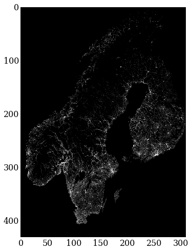
Here I import an map with the population density of the Nordic countries and downsample it to make the solving time resonably fast.

from PIL import Image
img = Image.open('popdens2.png')
img = img.resize((img.size[0]/2,img.size[1]/2)) 
img = 255 - np.asarray(img)
imgplot = plt.imshow(img)
imgplot.set_interpolation('nearest')

png

Population density in the Nordic countries (Denmark is missing)

Our $S$ matrix, the susceptible individuals should be something like the population density. The infected $I$ is for now just zeros. But let’s put a patient zero somewhere in Stockholm.

S_0 = img[:,:,1]
I_0 = np.zeros_like(S_0)
I_0[309,170] = 1 # patient zero

Nobodys dead, yet. So lets put $R$ to zeroes too.

R_0 = np.zeros_like(S_0)

Now set some initial values of how long the simulation is to be run and so on.

T = 900                         # final time
dt = 1                          # time increment
N = int(T/dt) + 1               # number of time-steps
t = np.linspace(0.0, T, N)      # time discretization

# initialize the array containing the solution for each time-step
u = np.empty((N, 3, S_0.shape[0], S_0.shape[1]))
u[0][0] = S_0
u[0][1] = I_0
u[0][2] = R_0

We need to make a custom colormap so that the infected matrix can be overlayed on the map.

import matplotlib.cm as cm
theCM = cm.get_cmap("Reds")
theCM._init()
alphas = np.abs(np.linspace(0, 1, theCM.N))
theCM._lut[:-3,-1] = alphas

And we sit back and enjoy…

for n in range(N-1):
    u[n+1] = euler_step(u[n], f, dt)

Not let’s render some images and make a gif of it. Everybody loves gifs!

from images2gif import writeGif

keyFrames = []
frames = 60.0

for i in range(0, N-1, int(N/frames)):
    imgplot = plt.imshow(img, vmin=0, vmax=255)
    imgplot.set_interpolation("nearest")
    imgplot = plt.imshow(u[i][1], vmin=0, cmap=theCM)
    imgplot.set_interpolation("nearest")
    filename = "outbreak" + str(i) + ".png"
    plt.savefig(filename)
    keyFrames.append(filename)
  
images = [Image.open(fn) for fn in keyFrames]
gifFilename = "outbreak.gif"
writeGif(gifFilename, images, duration=0.3)
plt.clf()

alt text

The spread of infection as a gif. Even the Finns will succumb.

Look at that! The only safe place seem to be in the northern parts where it’s not so densly populated. Even Finland will at the end of the animation be infected. Now you know.

If you want to know more about solving differential equations I can warmly recommend Practical Numerical Methods with Python by @LorenaABarba. Here you’ll learn all the real numerical methods that should be used instead of the simple one in this post.

UPDATE: To play around for yourself, the Ipython notebook can be found here.