Mapping town names atomic parts in Sweden
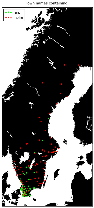
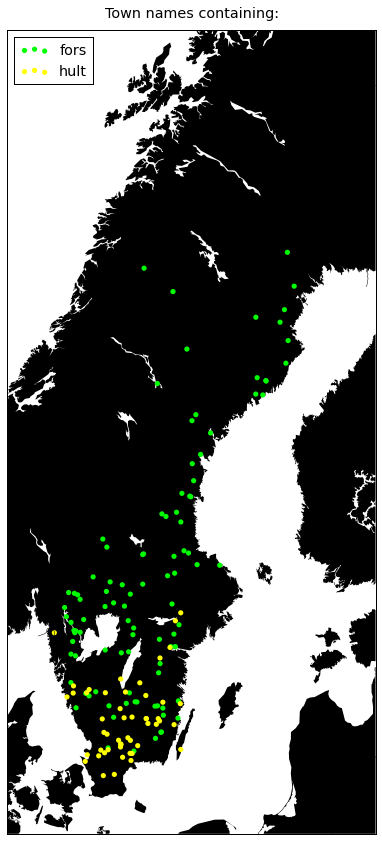
Many towns in Sweden share the same atomic parts in their names. -hult is common in Småland -arp is common in Skåne. I got curious of how they cluster geographically. Let’s load up a DataFrame with the positions of Swedish towns that I made by querying Google for the position of every Swedish town I could find on Wikipedia.
This notebook is also available as a Jupyter Notebook here if you want to execute the code yourself.
Scroll past the code if you’re only here for the maps.
import pandas as pd

df = pd.read_csv('swe_towns_latlon.csv', encoding='utf-8')
df['town'] = df['town'].str.lower()
And then do some crappy character n-gram extractions.
def find_features(s):
    feats = [s[i:i+7] for i in xrange(len(s)-6)]
    feats += [s[i:i+6] for i in xrange(len(s)-5)]
    feats += [s[i:i+5] for i in xrange(len(s)-4)]
    feats += [s[i:i+4] for i in xrange(len(s)-3)]
    feats += [s[i:i+3] for i in xrange(len(s)-2)]
    return feats

features = []
for town in df['town'].values:
    features.extend(find_features(town))
To be able to count the occurances.
features = list(set(features))
final_features = []
occurances = []

for feature in features:
    try:
        occurances.append(sum(df['town'].str.contains(feature)))
        final_features.append(feature)
    except:
        pass

df_features = pd.DataFrame({
    'feature': final_features,
    'occurances': occurances
})
So now we get interesting parts of town names. Sanity check (at least if you’re Swedish) is that sta, hult and so on are present.
print ", ".join(df_features.sort('occurances', ascending=False).head(100)['feature'].values)

sta, tor, ing, erg, nge, orp,  oc,  och , och , och, ch ,  och, vik, torp, ra , ber, ors, berg, und, sjö, tra, and, str, näs, ter, inge, stra, tad, stad, den, for, fors, mar, ken, sto, olm, ste, äst, storp, stor, lla, lle, all, dal, hol, ngs, holm, äll, lst, tra , ång, ers, orr, stra , red, ran, nda, arp, ham, ill, est, ung, äck, ten, ster, gen, jör, rby, jär, nne, cke, ult, amm, mma, lin, sun, ryd, ack, sby, äng, eby, byn, len, lan, sund, ling, ker, nna, mmar, löv, lun, ike, bäck, bro, tan, nga, bäc, ård, rst, tte
I went ahead and took out the ones I deemed interesting. Now let’s plot them to se how they group geographically.
from mpl_toolkits.basemap import Basemap
import matplotlib.pyplot as plt
from matplotlib import rcParams
rcParams['font.family'] = 'sans-serif'
rcParams['font.sans-serif'] = ['Helvetica Neue']
%matplotlib inline

def plot(data, mult=0.9):
    """ Take data with 'part-of-towns-name' and color and plot it. Use `mult` for easy scaling of plot """

    def get_coordinates(townpart):
        try:
            townpart = townpart.decode('utf-8')
        except:
            pass
        return df[df['town'].str.contains(townpart)]['lat'].values, df[df['town'].str.contains(townpart)]['lon'].values

    fig = plt.figure(figsize=(20*mult, 16*mult), dpi=200)

    m = Basemap(
        projection='merc',
        resolution='i',
        area_thresh=250,
        llcrnrlon=9.5,
        llcrnrlat=54.5,
        urcrnrlon=24.5,
        urcrnrlat=69.5
    )

    m.drawcoastlines(linewidth=0, color="#000000")
    m.drawcountries()
    m.drawstates()
    m.drawmapboundary()
    m.fillcontinents(color='black', lake_color='white', zorder=0)
    m.drawmapboundary(fill_color='white')
    title = plt.title(u'Town names containing:', fontsize=16*mult)
    title.set_y(1.01)

    for townpart in data.keys():
        lats, lons = get_coordinates(townpart)
        x, y = m(lons, lats)
        m.scatter(x, y, marker='o', s=30*mult, alpha=1, label=townpart, edgecolors='none', c=data[townpart])

    plt.legend(loc=2, fontsize=16*mult)
    plt.show()


plot({
    'arp': '#00ff00',
    'holm': '#ff0000',
})
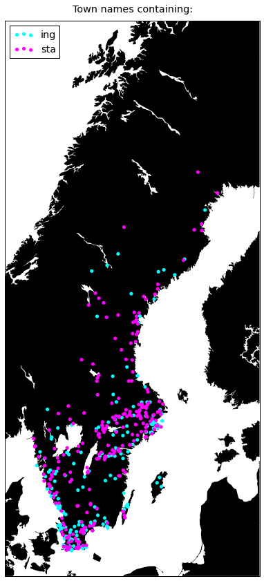
plot({
    'sta': '#ff00ff',
    'ing': '#00ffff',
})
plot({
    'hult': '#ffff00',
    'fors': '#00ff00',
})
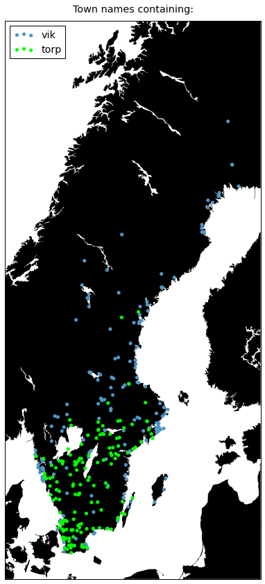
plot({
    'vik': '#4f96c5',
    'torp': '#00ff00',
})
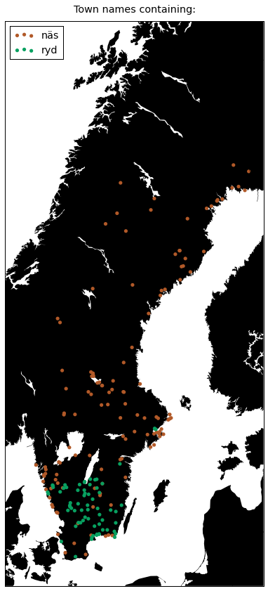
plot({
    u'näs': '#b15928',
    'ryd': '#08a060',
})
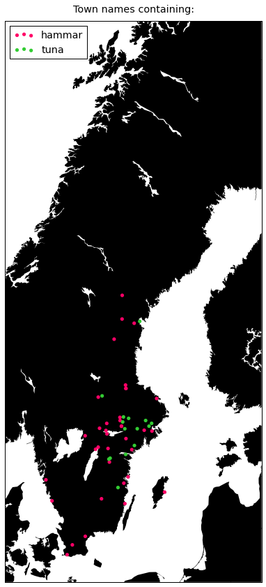
plot({
    'tuna': '#33cc33',
    'hammar': '#ff0066',
})
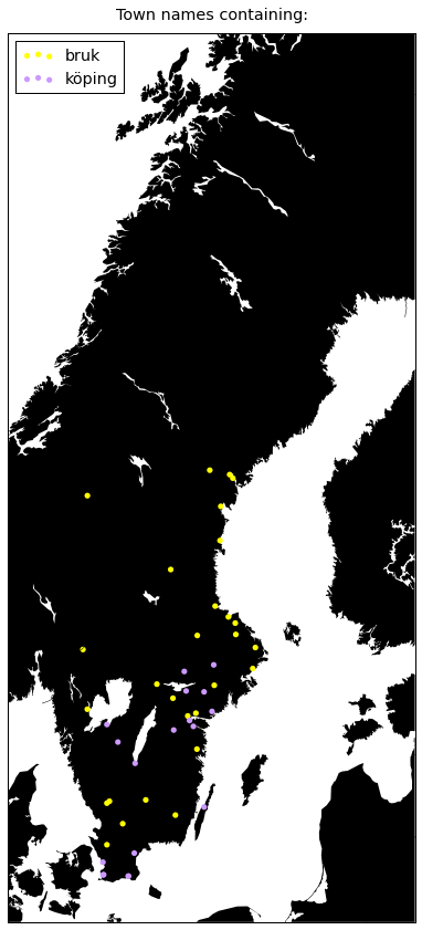
plot({
    u'köping': '#cc99ff',
    u'bruk': '#ffff00',
})
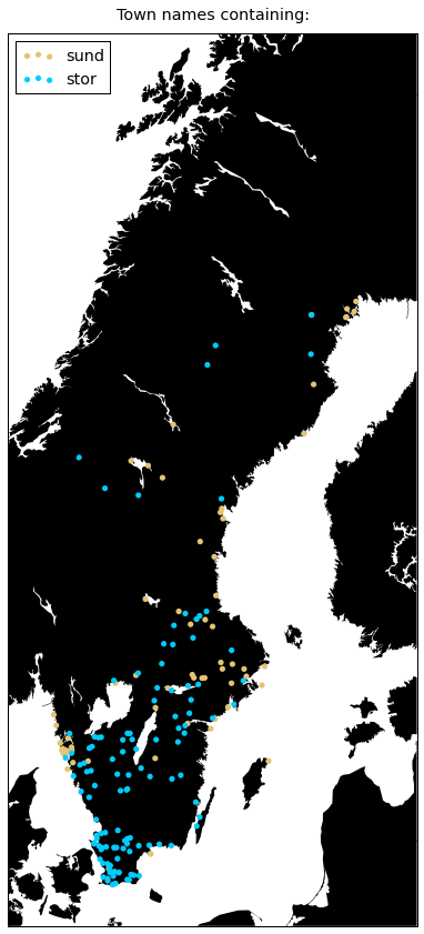
plot({
    'stor': '#00ccff',
    'sund': '#e3c471',
})
plot({
    'stad': '#ffcc00',
    'berg': '#9933ff',
})
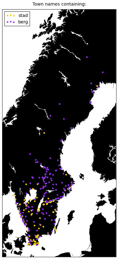
Berg is really common in the old mining regions called Bergslagen.
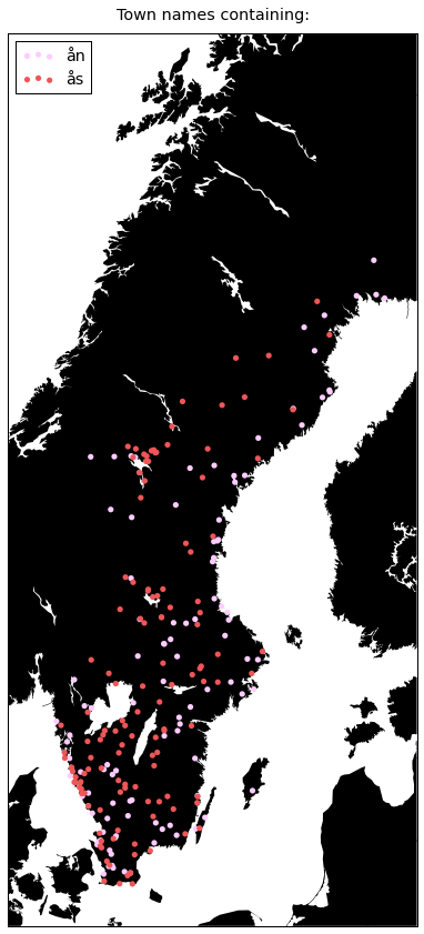
plot({
    u'ån': '#ffccff',
    u'ås': '#ee5657'
})