Polling is failing us: How to collect less biased data with computational methods
In the aftermath of the US elections it is clear that polling has it’s flaws. Pollsters are good at compensating for things like underrepresented minorities, picking fair samples and with the popularization of polls of polls — even aggregating all known data to get a bigger picture. Thanks to the latter, most people now even can relate to probability of winning instead of share of votes.
This is great. But one big bias in polling makes all this skewed. The fact that there is a established moral high ground. Voting against that is something that might have social implications. So a good proportion of people prompted in a poll will therefore not give a truthful answer.
This is clear from both the Swedish election 2014, Brexit and now also the 2016 US presidential election. The majority of polls underestimated the less socially favorable alternative.
| Referendum | Polls-of-polls 1 | Outcome | Abs. diff. | Rel. diff. |
|---|---|---|---|---|
| Sweden 2014 | 10 % Sweden Democrats2 | ~13 % | +3 % | +30 % |
| Brexit | ~49 % leave3 | ~52 % | +3 % | +6 % |
| US 2016 | ~44 % Trump4 | ~56 % | +12 % | +27 % |
1Normalized for decided voters. 2Boten Ada. 3Financial times. 4Electoral votes 938.com.
So how do you get people to answer truthfully? One classic method is a Randomized Response Model. In it’s most simple form (two outcomes of the question, like for example the US presidential election) the respondent is asked to
- First toss a coin.
- If heads: tell what presidential candidate she will vote for
- If tail
- Toss coin once again and say Clinton if heads and Trump if tail.
This gives the respondee the possibility to speak freely since the surveyor will not know if it’s an answer governed by chance or a truthful answer.
But what about the data? We can in fact still model the underlying percentage before the coin flips. We need more data since we are introducing noise. But it might be a small price to pay for unbiased data.
Let’s look at the different outcomes for this model.

From this graph we can make an expression for the probability of getting a Trump answer. If $P_T$ is the true proportion of that will vote for Trump, $T_O$ will be observed Trump answers.
Just for clarity sake, the corresponding expression for proportion observed Clinton votes is:
Now let’s create a Bayesian Markov chain Monte Carlo model out of this. First let’s generate 1000 true votes.
import pymc3 as pm
import numpy as np

N = 1000
true_p = 0.6
true_votes = np.random.choice([0, 1], size=(N,), p=[1-true_p, true_p])
The true votes is just an array looking something like [1 0 1 0 1 1 1 ... 0 0 1 0 1 0] with N entries. Given big enough N the percentage ones would be close to 60 % since that’s the percentage we choose for generating the random data.
Now starting from the true votes, we skew them in the same way as our algorithm would.
skewed_answers = true_votes.copy()
for i, vote in enumerate(skewed_answers):
    # If coin comes up heads - change answer
    if np.random.choice([0, 1], p=[.5, .5]) == 1:
        # Change to random flip of second coin
        skewed_answers[i] = np.random.choice([0, 1], p=[.5, .5])
Obviously we would not know the true votes in a real life situation, only the skewed_answers that’s now been generated.
Now that we have synthetic data let’s build a model that infers the true votes. This is heavily inspired by chapter 2 in Cam Davidson-Pilon’s great book Bayesian Methods for Hackers.
It works in a way that we construct a model that could have generated the data. And then gives it the data and asks questions about the variables in the model.
In this case $P_T$, the proportion of Trump voters is the variable we want to know about – but we create a model that given an (yet) unknown $P_T$ could generate the skewed data that we got. It follows the logic we just derived expressing the proportion observed Trump votes.
Now to the model
%matplotlib inline
import matplotlib.pyplot as plt
import seaborn as sns

with pm.Model() as model:

    # Proportion Trump defined as between 0 and 1
    P_T = pm.Uniform("prop_trump_votes", 0, 1)

    # Observed proportion follows this expression
    P_O = pm.Deterministic(
        "prop_skewed",
        0.5 * P_T + 0.25)

    # A Binomial generates ones and zeros
    T_O = pm.Binomial(
        "number_trump_votes", N,
        P_O, # by the observed probability
        observed=sum(skewed_answers))
    # and we also gave it the observed skewed votes
    # so it know what to optimize for.

    # Now we run the inference
    step = pm.Metropolis(vars=[P_T])
    trace = pm.sample(40000, step=step)
    burned_trace = trace[2500:]

# Visualizing the distribution of the true proportion P_T
sns.distplot(
    burned_trace["prop_trump_votes"],
    bins=30, label='Posterior distribution')

sns.plt.xlim(0, 1)
sns.plt.legend()
[-----------------100%-----------------] 40000 of 40000 complete in 3.2 sec
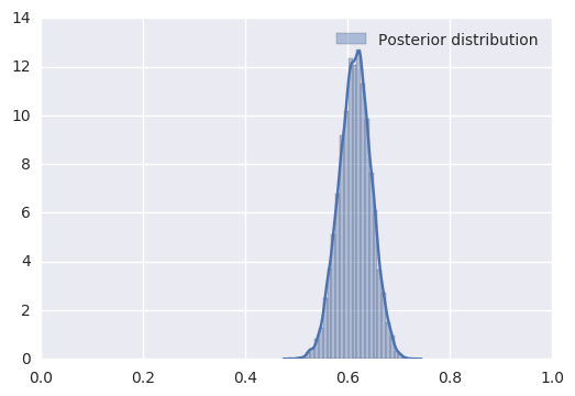
As you can see it’s not a clear answer saying 60 % as in true_p like the data we generated. We get a distribution of where the true proportion Trump voters $P_T$ lies because
- our method/algorithm introduced noise in the data
- and since there’s always a chance that the data would come up just by the random nature of the universe.
But from the graph, we can be quite confident that a larger proportion of the voters will choose Trump even with respecting the privacy of the respondents.
There are of course some problems with this method. Respondees could perhaps not understand what they are supposed to do in the flipping of coins here and there, and you need to collect more responses to battle the noise. But since it’s obvious that polling does not measure peoples true intentions in the case of a controversial alternative, data people needs to start thinking about alternative methods in understanding people.