Using ANNs on small data – Deep Learning vs. Xgboost
Andrew Beam does a great job showing that small datasets are not off limits for current neural net methods. If you use the regularisation methods at hand – ANNs is entirely possible to use instead of classic methods.
Let’s see how this holds up on up on some benchmark datasets.
%matplotlib inline
import numpy as np
import pandas as pd
import matplotlib.pyplot as plt
plt.style.use('ggplot')

seed = 123456
np.random.seed(seed)
Let’s start with the iris dataset that you nicely can pull with the pandas read_csv function right of the internets.
target_variable = 'species'
df = (
    pd.read_csv('https://gist.githubusercontent.com/curran/a08a1080b88344b0c8a7/raw/d546eaee765268bf2f487608c537c05e22e4b221/iris.csv')

    # Rename columns to lowercase and underscores
    .pipe(lambda d: d.rename(columns={
        k: v for k, v in zip(
            d.columns,
            [c.lower().replace(' ', '_') for c in d.columns]
        )
    }))
    # Switch categorical classes to integers
    .assign(**{target_variable: lambda r: r[target_variable].astype('category').cat.codes})
)
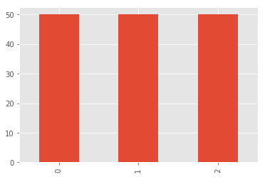
There’s three classes and 150 datapoints. Not really B̫͕̟̱I̜̼͈̖̫G͉ d̙͕a͇͍͕̝̟t̪̝̹̻͉̭ͅa.
df[target_variable].value_counts().sort_index().plot.bar()
We create a feature matrix X and a target y from the Pandas dataframe. And since an ANN needs the features to be normalized, let’s do some min-max-scaling before anything else.
y = df[target_variable].values
X = (
    # Drop target variable
    df.drop(target_variable, axis=1)
    # Min-max-scaling (only needed for the DL model)
    .pipe(lambda d: (d-d.min())/d.max()).fillna(0)
    .as_matrix()
)
We split into a training set and a test set.
from sklearn.metrics import accuracy_score
from sklearn.model_selection import train_test_split, cross_val_score

X_train, X_test, y_train, y_test = train_test_split(
    X, y, test_size=0.33, random_state=seed
)
Import some keras goodness (and perhaps run pip install keras first if you need it).
from keras.models import Sequential
from keras.callbacks import EarlyStopping, ModelCheckpoint
from keras.layers import Dense, Activation, Dropout
from keras import optimizers
And set up a thee layer deep and 128 wide net. Nothing fancy, not even sure this would qualify as deep learning – but throw in some dropout between them to help it to not overfit.
Learning rate for the optimization method Adam might be something to tune on other datasets but here 0.001 seems to work nicely.
m = Sequential()
m.add(Dense(128, activation='relu', input_shape=(X.shape[1],)))
m.add(Dropout(0.5))
m.add(Dense(128, activation='relu'))
m.add(Dropout(0.5))
m.add(Dense(128, activation='relu'))
m.add(Dropout(0.5))
m.add(Dense(len(np.unique(y)), activation='softmax'))

m.compile(
    optimizer=optimizers.Adam(lr=0.001),
    loss='categorical_crossentropy',
    metrics=['accuracy']
)
EarlyStopping helps us stop the training when the validation set is not improving any more – which helps us avoid overfitting. And to keep the checkpoint just before overfitting occurs, ModelCheckpoints let’s us save the best model before decline in validation set performance.
m.fit(
    # Feature matrix
    X_train,
    # Target class one-hot-encoded
    pd.get_dummies(pd.DataFrame(y_train), columns=[0]).as_matrix(),
    # Iterations to be run if not stopped by EarlyStopping
    epochs=200,
    callbacks=[
        # Stop iterations when validation loss has not improved
        EarlyStopping(monitor='val_loss', patience=25),
        # Nice for keeping the last model before overfitting occurs
        ModelCheckpoint(
            'best.model',
            monitor='val_loss',
            save_best_only=True,
            verbose=1
        )
    ],
    verbose=2,
    validation_split=0.1,
    batch_size=256,
)
# Load the best model
m.load_weights("best.model")

# Keep track of what class corresponds to what index
mapping = (
    pd.get_dummies(pd.DataFrame(y_train), columns=[0], prefix='', prefix_sep='')
    .columns.astype(int).values
)
y_test_preds = [mapping[pred] for pred in m.predict(X_test).argmax(axis=1)]
Now we can assess the performance on the test set. Below is a confusion matrix showing all predictions held up to reality.
pd.crosstab(
    pd.Series(y_test, name='Actual'),
    pd.Series(y_test_preds, name='Predicted'),
    margins=True
)
| Predicted | 0 | 1 | 2 | All |
|---|---|---|---|---|
| Actual | ||||
| 0 | 18 | 0 | 0 | 18 |
| 1 | 0 | 16 | 0 | 16 |
| 2 | 0 | 0 | 16 | 16 |
| All | 18 | 16 | 16 | 50 |
print 'Accuracy: {0:.3f}'.format(accuracy_score(y_test, y_test_preds))
Accuracy: 1.000
Actually a perfect score. We will now do the same with an good old xgboost (conda install xgboost) with the nice sklearn api.
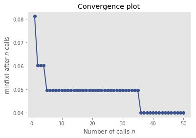
Finding the right hyperparameters is a task well suited for an Bayesian approach that can test the alternatives in an effective way without any gradient. GridSearch and such takes alot of time – this way we instead give it a parameter space and a “budget”. It will then in it’s most cost effective way test the hyperparameters of xgboost under those constraints.
from xgboost.sklearn import XGBClassifier

params_fixed = {
    'objective': 'binary:logistic',
    'silent': 1,
    'seed': seed,
}

# The space to search
space = {
    'max_depth': (1, 5),
    'learning_rate': (10**-4, 10**-1),
    'n_estimators': (10, 200),
    'min_child_weight': (1, 20),
    'subsample': (0, 1),
    'colsample_bytree': (0.3, 1)
}

reg = XGBClassifier(**params_fixed)

def objective(params):
    """ Wrap a cross validated inverted `accuracy` as objective func """
    reg.set_params(**{k: p for k, p in zip(space.keys(), params)})
    return 1-np.mean(cross_val_score(
        reg, X_train, y_train, cv=5, n_jobs=-1,
        scoring='accuracy')
    )
For this we use skopt (pip install scikit-optimize). I’ve given it 50 iterations to explore the hyperparameter space. Might be some more performance to squeeze out, but probably not.
from skopt import gp_minimize
res_gp = gp_minimize(objective, space.values(), n_calls=50, random_state=seed)
best_hyper_params = {k: v for k, v in zip(space.keys(), res_gp.x)}

print "Best accuracy score =", 1-res_gp.fun
print "Best parameters =", best_hyper_params
Best accuracy score = 0.96
Best parameters = {'colsample_bytree': 1.0, 'learning_rate': 0.10000000000000001, 'min_child_weight': 5, 'n_estimators': 45, 'subsample': 1, 'max_depth': 5}
from skopt.plots import plot_convergence
plot_convergence(res_gp)
Now let’s fix these hyperparameters and evaluate on the test set. This is exactly the same test set as Keras got to be clear.
params = best_hyper_params.copy()
params.update(params_fixed)

clf = XGBClassifier(**params)
clf.fit(X_train, y_train)
y_test_preds = clf.predict(X_test)
pd.crosstab(
    pd.Series(y_test, name='Actual'),
    pd.Series(y_test_preds, name='Predicted'),
    margins=True
)
| Predicted | 0 | 1 | 2 | All |
|---|---|---|---|---|
| Actual | ||||
| 0 | 18 | 0 | 0 | 18 |
| 1 | 0 | 15 | 1 | 16 |
| 2 | 0 | 2 | 14 | 16 |
| All | 18 | 17 | 15 | 50 |
print 'Accuracy: {0:.3f}'.format(accuracy_score(y_test, y_test_preds))
Accuracy: 0.940
The deep (?) net got all datapoints right while xgboost missed three of them. On the other hand if you change the seed and rerun the code it might as well be xgboost coming up on top so I wouldn’t read to much into it.
Let’s generalize the code above so that we can plug in any dataset of choosing and see if this holds for harder problems. While we’re at it, I’ve added a boostrap on the accuracy statistic to give a feel about the uncertanty. I’ve put the code in this gist since it’s more or less just a repetition of the code above.
Telecom churn dataset (n=2325)
compare_on_dataset(
    'https://community.watsonanalytics.com/wp-content/uploads/2015/03/WA_Fn-UseC_-Telco-Customer-Churn.csv?cm_mc_uid=06267660176214972094054&cm_mc_sid_50200000=1497209405&cm_mc_sid_52640000=1497209405',
    target_variable='churn',
    lr=0.0005,
    patience=5
)
ANN
| Predicted | 0 | 1 | All |
|---|---|---|---|
| Actual | |||
| 0 | 1478 | 270 | 1748 |
| 1 | 218 | 359 | 577 |
| All | 1696 | 629 | 2325 |
Accuracy: 0.790
Boostrapped accuracy 95 % interval 0.770223752151 0.809810671256
Xgboost
| Predicted | 0 | 1 | All |
|---|---|---|---|
| Actual | |||
| 0 | 1563 | 185 | 1748 |
| 1 | 265 | 312 | 577 |
| All | 1828 | 497 | 2325 |
Accuracy: 0.806
Boostrapped accuracy 95 % interval 0.78743545611 - 0.825301204819
Churn is a bit harder problem, but both methods do well though.
Three class wine dataset (n=59)
compare_on_dataset(
    'https://gist.githubusercontent.com/tijptjik/9408623/raw/b237fa5848349a14a14e5d4107dc7897c21951f5/wine.csv',
    target_variable='wine',
    lr=0.001
)
ANN
| Predicted | 0 | 1 | 2 | All |
|---|---|---|---|---|
| Actual | ||||
| 0 | 18 | 1 | 0 | 19 |
| 1 | 0 | 19 | 0 | 19 |
| 2 | 0 | 0 | 21 | 21 |
| All | 18 | 20 | 21 | 59 |
Accuracy: 0.983
Boostrapped accuracy 95 % interval 0.931034482759 1.0
Xgboost
| Predicted | 0 | 1 | 2 | All |
|---|---|---|---|---|
| Actual | ||||
| 0 | 19 | 0 | 0 | 19 |
| 1 | 0 | 19 | 0 | 19 |
| 2 | 0 | 0 | 21 | 21 |
| All | 19 | 19 | 21 | 59 |
Accuracy: 1.000
Boostrapped accuracy 95 % interval 1.0 1.0
A very easy dataset that both methods have no problem with. Since the sample size is so small the boostrap will not be much of use to us here.
German Credit Data (n=1000)
compare_on_dataset(
    'https://onlinecourses.science.psu.edu/stat857/sites/onlinecourses.science.psu.edu.stat857/files/german_credit.csv',
    target_variable='creditability',
    lr=0.001,
    patience=5
)
ANN
| Predicted | 0 | 1 | All |
|---|---|---|---|
| Actual | |||
| 0 | 43 | 45 | 88 |
| 1 | 28 | 214 | 242 |
| All | 71 | 259 | 330 |
Accuracy: 0.779
Boostrapped accuracy 95 % interval 0.727272727273 0.830303030303
Xgboost
| Predicted | 0 | 1 | All |
|---|---|---|---|
| Actual | |||
| 0 | 37 | 51 | 88 |
| 1 | 25 | 217 | 242 |
| All | 62 | 268 | 330 |
Accuracy: 0.770
Boostrapped accuracy 95 % interval 0.715151515152 0.824242424242
So sometimes the ANN comes out on top, and sometime it’s xgboost. I think it’s fair to say that ANNs, controlled for overfitting/overtraining works kinda great even small data. At least pair with xgboost.
And the necessary hyperparameter tuning of xgboost is a pain since it really takes time. On these datasets, training the ANN takes no time at all. So let’s see if ANNs will start to eat small data also anytime soon.