Gender bias in language – analysis of bigrams in a news text corpus
Julia Silge recently wrote a blog post about co-occurances of words together with gendered pronouns. This made me dig up some old code that did the same, but with the difference that it also extends to gendered names besides pronouns. The data is a corpus of Swedish news texts, and I’ve used name statistics from Sweden Statistics (SCB) to parse out what names are male and female.
So let’s hack up a naive bookkeeping code to count all bigrams containing he/she/male_name/female_name. My corpus has already replaced all names with female_name/male_name since that’s what my gender monitor does. I’ll use textacy for tokenization that uses the really fast spaCy behind the hoods. That said, this still takes some time to run. I did start to redo it in dask, but I realized that would take more time than to just let it run (see appropiate xkcd).
# For my unorthodox csv
import sys, csv
csv.field_size_limit(sys.maxsize)

# A counter for female and male connections
from collections import Counter
cnt = {'he': Counter(), 'she': Counter()}

import textacy
for d in textacy.fileio.read.read_csv('news_corpus.csv'):

    # Extract tokens
    doc = textacy.Doc(d[0].lower(), lang=u'sv')

    # Extract bigrams
    ngrams = textacy.extract.ngrams(
        doc, n=2,
        filter_stops=False,
        filter_punct=False,
        filter_nums=False)

    # Bookkeeping for all bigram findings
    for gram in ngrams:

        t0 = str(gram[0]) # First token in bigram
        t1 = str(gram[1]) # Second token in bigram

        if t0 == 'han':
            cnt['he'][t1] += 1
        elif t1 == 'han':
            cnt['he'][t0] += 1

        elif str(t0) == 'male_name':
            cnt['he'][t1] += 1
        elif str(t1) == 'male_name':
            cnt['he'][t0] += 1

        elif str(t0) == 'hon':
            cnt['she'][t1] += 1
        elif str(t1) == 'hon':
            cnt['she'][t0] += 1

        elif str(t0) == 'female_name':
            cnt['she'][t1] += 1
        elif str(t1) == 'female_name':
            cnt['she'][t0] += 1
Now cnt['he'] and cnt['she'] holds the frequencies for co-occurances of he and vice versa for she. But we want it to be in percent so we can compare. About 75 % of all mentions in news media are of males, so we need to remove this bias to answer the question “How more often is word X used together with he rather than she”.
So let’s transform to percent and throw away some of the long tail to remove noise (keeping everything under percentile 95).
import pandas as pd
import numpy as np
he = (
    pd.DataFrame()
    .from_dict(cnt['he'], orient='index')
    .rename(columns={0: 'he'})
    .pipe(lambda d: d[d.he > d.quantile(.95)['he']])
    .pipe(lambda d: d/d.sum())
    .sort_values('he', ascending=False)
)

she = (
    pd.DataFrame()
    .from_dict(cnt['she'], orient='index')
    .rename(columns={0: 'she'})
    .pipe(lambda d: d[d.she > d.quantile(.95)['she']])
    .pipe(lambda d: d/d.sum())
    .sort_values('she', ascending=False)
)
For the male connected words that’s,
he.head(5)
| he | |
|---|---|
| . | 0.487862 |
| har | 0.066698 |
| är | 0.054389 |
| var | 0.033257 |
| – | 0.020974 |
and for female connected words,
she.head(5)
| she | |
|---|---|
| . | 0.499746 |
| har | 0.073374 |
| är | 0.061925 |
| var | 0.027128 |
| > | 0.019119 |
holding what we are interested in. Except the punctuation, and also some emails.
odds = (
    # Joining
    he.merge(she, left_index=True, right_index=True)
    # Calc logodds
    .assign(logodds=lambda r: np.log2(r['she'] / r['he']))
    # Removing punctuation
    .pipe(lambda d: d[d.index.str.len() > 1])
    # Removing emails
    .pipe(lambda d: d[~d.index.str.contains('@')])
    .pipe(lambda d: d[~d.index.str.contains('kundservice')])
    .sort_values('logodds', ascending=True)
)
Now let’s compare the ratios to find out what words are more used in connection to she and female names. We do this by joining/merging the he and she DataFrames. Taking the log of this ratio conviniently centers the bias around zero – positive meaning skewed towards females and negative towards male.
Most male connected
odds.query('logodds < 0').head(50)
| he | she | logodds | |
|---|---|---|---|
| index | |||
| could | 0.002774 | 0.001636 | -0.761978 |
| speaks | 0.002140 | 0.001354 | -0.660601 |
| argues | 0.003989 | 0.002594 | -0.620557 |
| explains | 0.002985 | 0.002030 | -0.555968 |
| said | 0.004411 | 0.003046 | -0.534531 |
| adds | 0.002325 | 0.001636 | -0.507164 |
| wanted | 0.004015 | 0.002876 | -0.481216 |
| gave | 0.001691 | 0.001354 | -0.320751 |
| knows | 0.002087 | 0.001692 | -0.302604 |
| continues | 0.003408 | 0.002764 | -0.302231 |
| was | 0.033257 | 0.027128 | -0.293883 |
| says | 0.005442 | 0.004455 | -0.288434 |
| saying | 0.017143 | 0.014100 | -0.282004 |
| saw | 0.001875 | 0.001579 | -0.248106 |
| can | 0.005521 | 0.004681 | -0.238034 |
| wrote | 0.003091 | 0.002651 | -0.221490 |
| – | 0.020974 | 0.018668 | -0.168022 |
| mentions | 0.002008 | 0.001805 | -0.153641 |
| started | 0.001796 | 0.001636 | -0.135196 |
| considers | 0.004675 | 0.004286 | -0.125392 |
| had | 0.016668 | 0.015961 | -0.062552 |
| sees | 0.005943 | 0.005753 | -0.047070 |
| belives | 0.006102 | 0.006035 | -0.015996 |
| wants | 0.011728 | 0.011618 | -0.013629 |
And positive gives skew towards females.
Most female connected
odds.query('logodds > 0').tail(50)
| he | she | logodds | |
|---|---|---|---|
| index | |||
| takes | 0.003249 | 0.003384 | 0.058662 |
| come | 0.003830 | 0.004004 | 0.064124 |
| calls | 0.001453 | 0.001523 | 0.067814 |
| comes | 0.004253 | 0.004512 | 0.085297 |
| did | 0.002298 | 0.002482 | 0.110774 |
| means | 0.012019 | 0.013141 | 0.128750 |
| ska | 0.003698 | 0.004061 | 0.134928 |
| has | 0.066698 | 0.073374 | 0.137624 |
| notes | 0.003117 | 0.003440 | 0.142380 |
| goes | 0.001664 | 0.001861 | 0.161400 |
| pekar | 0.003196 | 0.003609 | 0.175423 |
| must | 0.001796 | 0.002030 | 0.176748 |
| became | 0.007370 | 0.008347 | 0.179618 |
| is | 0.054389 | 0.061925 | 0.187220 |
| holds | 0.001189 | 0.001354 | 0.187396 |
| got | 0.006551 | 0.007896 | 0.269373 |
| tells | 0.010170 | 0.012351 | 0.280359 |
| would | 0.003328 | 0.004061 | 0.286931 |
| took | 0.003011 | 0.003722 | 0.305790 |
| gets | 0.004042 | 0.005019 | 0.312632 |
| shows | 0.001902 | 0.002369 | 0.316679 |
| went | 0.002589 | 0.003271 | 0.337557 |
| ” | 0.013815 | 0.018047 | 0.385547 |
| write | 0.005415 | 0.007163 | 0.403491 |
| does | 0.002853 | 0.003779 | 0.405488 |
| thinks | 0.004834 | 0.006429 | 0.411476 |
| as | 0.002430 | 0.003271 | 0.428705 |
| dies | 0.001030 | 0.001410 | 0.452740 |
| describes | 0.003698 | 0.005076 | 0.456856 |
| told | 0.001294 | 0.001805 | 0.479576 |
| born | 0.001479 | 0.002087 | 0.496385 |
| laughs | 0.000898 | 0.001297 | 0.530385 |
| lets | 0.000925 | 0.001354 | 0.549966 |
| feels | 0.001347 | 0.001974 | 0.551144 |
| and | 0.003381 | 0.005132 | 0.602081 |
| sits | 0.001875 | 0.002876 | 0.616964 |
| gives | 0.001691 | 0.002764 | 0.708996 |
| asked | 0.000766 | 0.001297 | 0.759867 |
| remembers | 0.000819 | 0.001410 | 0.783946 |
| lifts | 0.001242 | 0.002200 | 0.825100 |
| lives | 0.001294 | 0.002425 | 0.905841 |
| becomes | 0.001426 | 0.004230 | 1.568217 |
Pick out the most skewed words for plotting
headsntails = pd.concat([
    odds.head(30).query('logodds < 0'),
    odds.tail(30).query('logodds > 0')
], axis=0)

# Some styling
%matplotlib inline
%config InlineBackend.figure_formats = {'png', 'retina'}
import seaborn as sns
import matplotlib.pyplot as plt
sns.set_palette("Paired", 15, .75)
sns.set_context("notebook", font_scale=1.2, rc={"lines.linewidth": 1.2})
sns.set_style("whitegrid")
custom_style = {
            'grid.color': '0.7',
            'grid.linestyle': '--',
            'grid.linewidth': 0.5,
}
sns.set_style(custom_style)

f, ax = plt.subplots(figsize=(8, 12))
x = [s.decode('utf-8') for s in headsntails['logodds'].index]
y = headsntails['logodds'].values

sns.barplot(y, x, palette="RdBu_r", ax=ax)

labels = [
    '{}x'.format(round(2**item, 1))
    for item in ax.get_xticks()
]
ax.set_xticklabels(labels)
ax.set_xlabel("Female usage")

for bar in ax.patches:
    smaller = 0.3
    height = bar.get_height()
    bar.set_height(height*smaller)
    move = height*(1-smaller)
    y = bar.get_y()
    bar.set_y(y+move)

# Finalize the plot
sns.despine(offset=5)
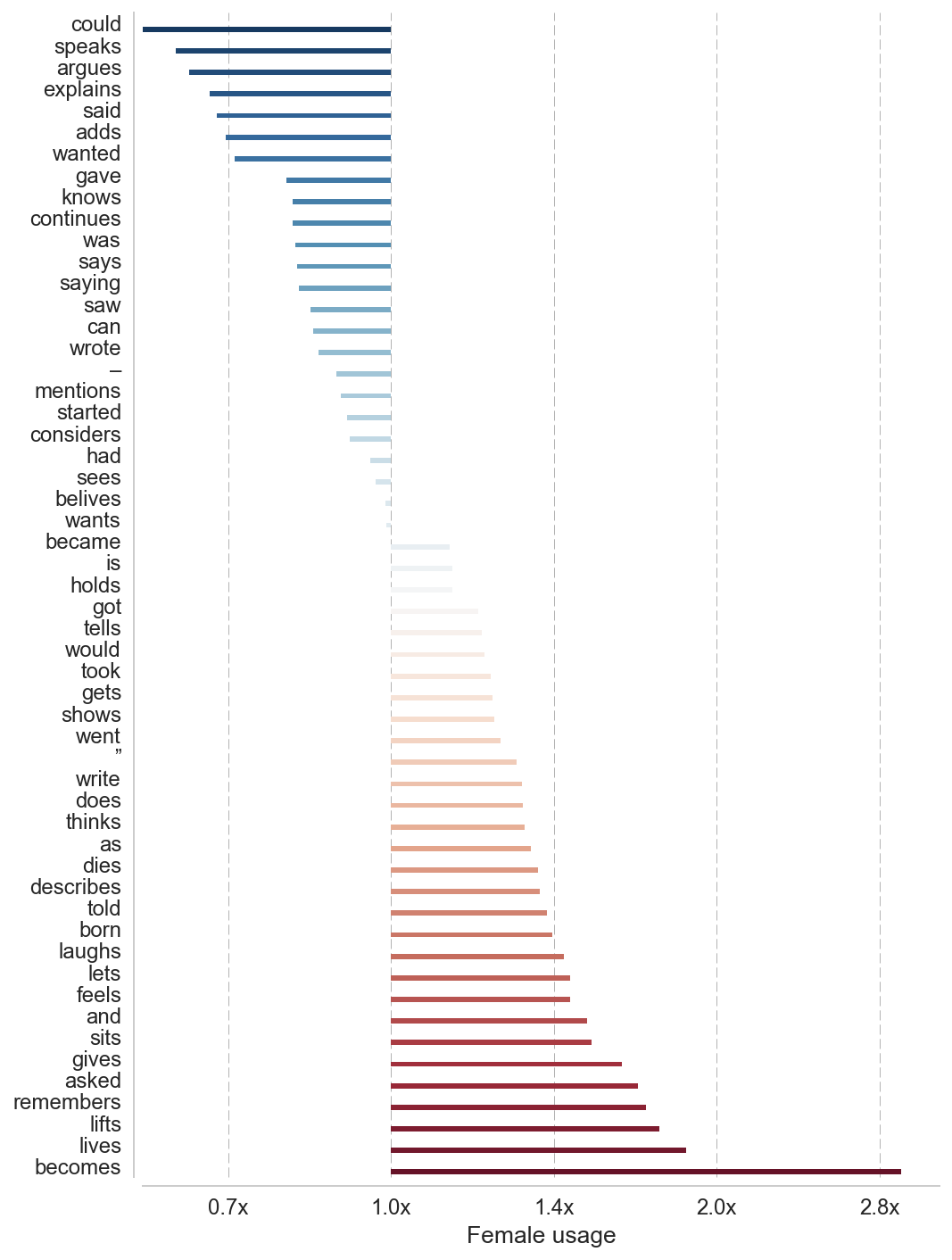
So men speaks, explains, says, thinks, [speaking punctuation] and statues. While women tells, describes, remembers, feels, live, recieves and sits. It’s clear that language is a mirror of what kind of values our society holds. Men are in news texts, other than just in real numbers more present – more in focus. More active and in the role as an expert. SAD!